Conditional formatting charts in excel
Although Excel ships with many conditional formatting presets these are limited. Progress doughnut charts have become.

Moving X Axis Labels At The Bottom Of The Chart Below Negative Values In Excel Pakaccountants Com Excel Excel Tutorials Chart
Here we have a table that shows monthly sales figures for a group of sales people.

. Conditional formatting rules are evaluated in order. Numbers that fall within a certain range ex. Besides background colors the Clear Conditional Formatting feature of Professor Excel Tools keeps all other common types of cell formatting font colors border etc.
Click OK then OK again to return to the Conditional Formatting Rules Manager. IFANDB45 B4. On the Excel Ribbon click the Home tab.
In the Ribbon select Home Conditional Formatting New Rule. It is pretty easy to implement. Conditional formatting allows you to automatically apply formattingsuch as colors icons and data barsto one or more cells based on the cell valueTo do this youll need to create a conditional formatting ruleFor example a conditional formatting rule might be.
Click on the Conditional Formatting icon in the ribbon from the Home menu. A common use case of conditional formatting is to highlight values in a set of data. In the New Formatting Rule dialog select Use a formula to determine which cells to format in Select a Rule Type section then choose one formula as you need to type in Format values where this formula is true text box.
Highlight Rows With Conditional Formatting IF Function. Click Apply to apply the formatting to your selected range and click Close. Enter the value 80 and select a formatting style.
Select and right-click the range where you want to paste the formatting rule B3B10 2 click Paste special and 3 choose Paste conditional formatting only. Conditional Formatting for Blank Cells is the function in excel that is used for creating inbuilt or customized formatting. How to Apply Conditional Formatting for Blank Cells.
Click Highlight Cells Rules Greater Than. To highlight a row depending on the value contained in a cell in the row with conditional formatting you can use the IF Function within a Conditional Formatting rule. For each cell in the range B5B12 the first formula is evaluated.
Excel Conditional Formatting for Blank Cells. Right-click a cell with a conditional formatting rule and click Copy or use the keyboard shortcut CTRL C. A2.
As a result the formatting rule is applied to the entire data. Select the range you want to apply formatting to. Select the Color Scales from the drop-down menu.
In the Ribbon select Home Conditional Formatting New Rule. For example you can create a rule that highlights cells that meet certain criteria. Download the Excel File.
Every cell in the range selected where the date in that cell is greater than the date in cell H8 will have its background color changed to orange. To see the existing Conditional Formatting Rules follow these steps. The Excel OR function returns TRUE if any given argument evaluates to TRUE and returns FALSE if all supplied arguments evaluate to FALSE.
Click OK then OK again to return to the Conditional Formatting Rules. Select the range you want to apply formatting to. Excel changes the format of cell A1 automatically.
We will apply conditional formatting so that the color of the circle changes as the progress changes. This article shows how to highlight rows column differences missing values and how to build Gantt charts and search boxes with conditional formatting. Select the range you want to apply formatting to.
Conditional formatting is a very popular feature of Excel and is usually used to shade cells with different colors based on criteria that the user defines. Heres the Excel workbook that I use in the video. Click OK then OK again to.
Excel Conditional Formatting allows you to define rules which determine cell formatting. In the list of conditional formatting options click Data Bars and then click one of the Data Bar options -- Gradient Fill or Solid Fill. Apply to More Cells by Copy-Pasting.
Click this link to see many more conditional formatting examples. Select Use a formula to determine which cells to format and enter the formula. Excel highlights the cells that are greater than 80.
Select the date column and click Home Conditional Formatting New Rule see screenshot. Today lets look at how to use conditional formatting to make your checklists better. There are 12 Color Scale options with different color variations.
This option is available in the Home Tab in the Styles group in Microsoft Excel. And if youre familiar with the MATCH Function youll know that it returns the position of a value in a list and in this example that could be. In this project you will learn how to analyze data and identify trends using a variety of tools in Microsoft Excel.
On the Ribbon click the Home tab and then in the Styles group click Conditional Formatting. We can apply the idea of conditional formatting to column charts by using multiple data series because the Excel feature applies only to cells not charts. If the value is less than 2000 color the cell red.
A more powerful way to apply conditional formatting is formulas because formulas allow you to apply rules based on any logic you want. For example an orange fill color. In the Ribbon select Home Conditional Formatting New Rule.
In this article we will learn how to color rows based on text criteria we use the Conditional Formatting option. Select the range of Speed values C2C9. Click Conditional Formatting then click Manage.
Select the cells you want to add the conditional formatting click Home Conditional Formatting New Rule. See Conditional Formatting Rules. Conditional formatting is applied with rules.
In the New Formatting Rule dialog box click Use a formula to determine which cells to format option in the Select a Rule Type list box and then enter this formula. Select a cell in the Excel table heading row. Conditional Formatting in Excel is used to highlight the data on the basis of some criteria.
The color on the top of the icon will apply to the highest values. See tips below The selected cells now show Data Bars along with the original numbers. Select Use a formula to determine which cells to format and enter the following formula.
On the Home tab in the Styles group click Conditional Formatting. Now if you remember my post from a couple of weeks ago with a similar example youll recall that I said Conditional Formatting formulas must always evaluate to TRUE or FALSE or their numeric equivalents of 1 and 0. The monthly sales quota is 5000 so lets use conditional formatting to highlight monthly sales numbers that are below that value.
Conditional formatting step by step. Go to the worksheet named Example. For example to test A1 for either x or y use ORA1xA1y.
This chart displays a progress bar with the percentage of completion on a single metric. From this we can highlight the duplicate color the cell as per different value ranges etc. Creating a heat map.
With conditional formatting you can define rules to highlight cells using a range of color scales and icons and. This technique just uses a doughnut chart and formulas. We create short videos and clear examples of formulas functions pivot tables conditional formatting and charts.
IFB45TRUEFALSE Click the Format button and select your desired formatting. Conditional formatting and charts are two tools that focus on highlighting and representing data in a visual form. Just select the cells you want to remove the rules from go to the Professor Excel ribbon and click on Clear Cond.
The top 10 items in a list. It would be difficult to see various. Change the value of cell A1 to 81.
Download it and follow along. We create short videos and clear examples of formulas functions pivot tables conditional formatting and charts.

Info Graphics Rag Conditional Formatting In 3d Chart Youtube Chart Infographic Excel Dashboard Templates

Make Waffle Charts In Excel Using Conditional Formatting How To Pakaccountants Com Excel Microsoft Excel Tutorial Excel Hacks

Conditional Formatting Intersect Area Of Line Charts Line Chart Chart Intersecting

Charts In Excel Excel Tutorials Chart Excel Templates

Make Waffle Charts In Excel Using Conditional Formatting How To Pakaccountants Com Excel Excel Tutorials Excel Hacks

Conditional Formatting Rule Order For Task Checklist Microsoft Excel Tutorial Excel Excel Templates Project Management

Rag Conditional Formatting In Progress Circle Chart Progress Excel Rag

Basic Conditional Formatting In Excel Access Using A Sales Example Exceldemy Excel Tutorials Excel Microsoft Excel

Conditional Formatting Of Lines In An Excel Line Chart Using Vba Excel Chart Line Chart

Making A Slope Chart Or Bump Chart In Excel How To Pakaccountants Com Microsoft Excel Tutorial Excel Tutorials Excel

Best Charts To Show Done Against Goal Excel Charts Excel Excel Templates Chart

Make Waffle Charts In Excel Using Conditional Formatting How To Pakaccountants Com Mobile News Excel Microsoft Excel Tutorial
Create Charts With Conditional Formatting

Excel Magic Trick 626 Time Gantt Chart Conditional Formatting Data Validation Custom Formulas Gantt Chart Excel Gantt Chart Templates
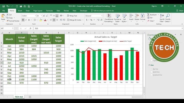
Tech 013 Create A Bar Chart With Conditional Formatting In Excel Youtube Excel Calendar Content Calendar Template Excel Calendar Template

Excel Conditional Formatting In Depth Excel Tutorials Excel Text Symbols

Conditional Formatting Of Excel Charts Peltier Tech Blog Excel Spreadsheets Excel Bar Graphs